QAOA
Similar to VQE, QAOA in Divi operates in multiple modes: a single-instance mode and a partitioning mode. The single-instance mode can be used to find a solution to a single graph-based or QUBO-based optimization problem. The partitioning mode is more specialized, focusing on solving larger, less tractable problems through a divide-and-conquer approach.
Single-instance QAOA
The QAOA constructor expects a QAOAProblem instance that encapsulates the problem definition — cost Hamiltonian, mixer, decoder, and recommended initial state. Divi provides concrete problem classes for common use cases.
A user can optionally override the initial state by passing an InitialState instance (e.g., ZerosState(), SuperpositionState()). By default, each problem class provides its own recommended initial state.
In addition, a user can determine how many layers of the QAOA ansatz to apply.
Finally, the solution of the QAOA problem can be accessed through the solution variable, which, based on the problem
at hand, would have different formats. For a graph problem, it will contain a set of node IDs that correspond to one
of the partitions of the solution. For QUBO optimization, it will return the solution bitstring as a list of 1’s and 0’s.
Graph Problems
Divi includes built-in support for several common graph-based optimization problems via concrete problem classes in divi.qprog.problems:
| Problem Class | Description |
|---|---|
MaxCliqueProblem |
Finds the largest complete subgraph where every node is connected to every other. |
MaxIndependentSetProblem |
Finds the largest set of vertices with no edges between them. |
MaxWeightCycleProblem |
Identifies a cycle with the maximum total edge weight in a weighted graph. |
MaxCutProblem |
Divides a graph into two subsets to maximize the sum of edge weights between them. |
MinVertexCoverProblem |
Finds the smallest set of vertices such that every edge is incident to at least one selected vertex. |
For all problems with the exception of MaxCut, the constrained version of the Hamiltonian is available by passing the
keyword argument is_constrained=True to the problem constructor. Refer to the PennyLane documentation for more details.
The following is an example for finding the max-clique of the bull graph:
import networkx as nx

from divi.backends import MaestroSimulator
from divi.qprog import QAOA
from divi.qprog.problems import MaxCliqueProblem
from divi.qprog.optimizers import ScipyOptimizer, ScipyMethod

G = nx.bull_graph()

qaoa_problem = QAOA(
    MaxCliqueProblem(G, is_constrained=True),
    n_layers=2,
    optimizer=ScipyOptimizer(ScipyMethod.NELDER_MEAD),
    max_iterations=10,
    backend=MaestroSimulator(),
)

qaoa_problem.run()

losses = qaoa_problem.losses[-1]
print(f"Minimum Energy Achieved: {min(losses.values()):.4f}")

print(f"Total circuits: {qaoa_problem.total_circuit_count}")

print(f"Classical solution:{nx.algorithms.approximation.max_clique(G)}")
print(f"Quantum Solution: {set(qaoa_problem.solution)}")

qaoa_problem.draw_solution()
As you can see, Divi provides a visualization function after computing the solution. Running the code above will generate the following plot:
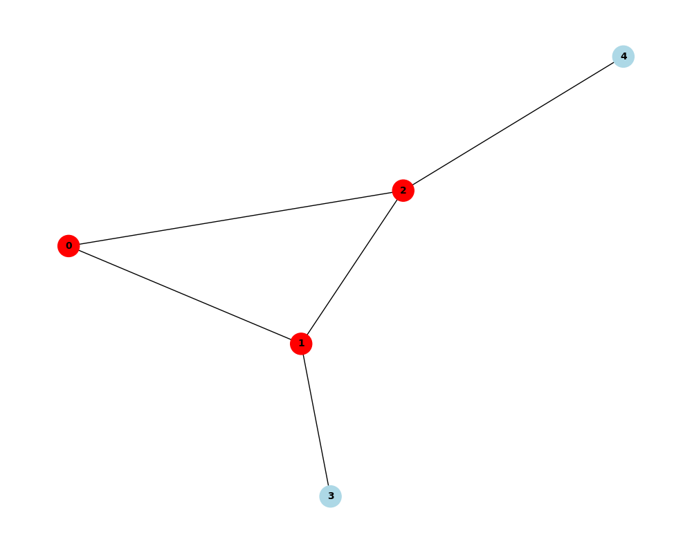
QAOA Max-Clique Solution on the Bull Graph
The solution can also be accessed through the solution property, which would generate the following list of node IDs corresponding to the Max-Clique:
>>> qaoa_problem.solution
[0, 1, 2]
QUBO-based Problems
Divi’s QAOA solver can also take a QUBO (Quadratic Unconstrained Binary Optimization) formulated problem instead of a graph. Divi supports the following QUBO input formats:
- NumPy array: A dense N×N matrix
- SciPy sparse matrix: For large, sparse QUBOs
- D-Wave’s
BinaryQuadraticModel: From thedimodlibrary
In contrast to graph-based QAOA instances, the solution format for QUBO-based QAOA instances is a binary numpy array representing the value for each variable in the original QUBO.
NumPy Array-based Input
For illustration purposes, we use D-Wave’s dimod
to generate a random QUBO.
from divi.qprog import QAOA
from divi.qprog.problems import BinaryOptimizationProblem
from divi.qprog.optimizers import ScipyOptimizer, ScipyMethod
from divi.backends import QoroService

# For generating the problem
import dimod

q_service = QoroService()

bqm = dimod.generators.randint(5, vartype="BINARY", low=-10, high=10, seed=1997)
qubo_array = bqm.to_numpy_matrix()

qaoa_problem = QAOA(
    BinaryOptimizationProblem(qubo_array),
    n_layers=2,
    optimizer=ScipyOptimizer(ScipyMethod.L_BFGS_B),
    max_iterations=5,
    backend=q_service,
)

qaoa_problem.run()
sol = qaoa_problem.solution
BinaryQuadraticModel Input
You can also pass a BinaryQuadraticModel directly:
import dimod
from divi.qprog import QAOA
from divi.qprog.problems import BinaryOptimizationProblem
from divi.qprog.optimizers import ScipyOptimizer, ScipyMethod
from divi.backends import MaestroSimulator

bqm = dimod.generators.randint(8, vartype="BINARY", low=-5, high=5, seed=42)

qaoa_problem = QAOA(
    BinaryOptimizationProblem(bqm),
    n_layers=2,
    optimizer=ScipyOptimizer(ScipyMethod.COBYLA),
    max_iterations=10,
    backend=MaestroSimulator(),
)

qaoa_problem.run()
sol = qaoa_problem.solution
QDrift Integration
QAOA supports QDrift as a trotterization strategy, which can reduce circuit depth for problems with many Hamiltonian terms. Pass a TrotterizationStrategy to enable it:
from divi.qprog import QAOA
from divi.qprog.problems import MaxCutProblem
from divi.hamiltonians import QDrift

qaoa_problem = QAOA(
    MaxCutProblem(G),
    n_layers=2,
    trotterization_strategy=QDrift(n_samples=50),
    optimizer=ScipyOptimizer(ScipyMethod.COBYLA),
    max_iterations=10,
    backend=MaestroSimulator(),
)
Partitioning QAOA
This example demonstrates how to use Divi’s PartitioningProgramEnsemble to solve a MaxCut problem on large graphs. Instead of executing a single large QAOA circuit, the graph is partitioned into smaller subgraphs (clusters), and individual QAOA instances are executed in parallel across these subgraphs, before aggregating the results, in a divide-and-conquer manner.
This enables scalable quantum optimization, even for graphs that exceed the size limits of a single quantum backend.
Configuring the Partitioning
The partitioning strategy is configured using the GraphPartitioningConfig class (passed to the problem constructor), which offers the following options:
-
max_n_nodes_per_cluster: This specifies the maximum number of nodes allowed in each subgraph or cluster. This is crucial for ensuring that each subproblem fits within the constraints of a single quantum backend. -
minimum_n_clusters: This parameter sets the minimum number of clusters to be created. -
partitioning_algorithm: A parameter that determines the algorithm used to partition the graph. The available options are:spectral: This refers to spectral clustering 1, an algorithm that uses the eigenvectors of the graph’s Laplacian matrix to partition the vertices. It’s known for producing high-quality partitions by minimizing the number of edges cut between the subgraphs. However, it might lead to unevenly sized partitions, based on the input graph.metis: Employs the popular METIS program 2 throughpy-metis. This algorithm generally generates more evenly sized partitions compared to spectral clustering.kernighan_linIteratively applies the classical Kernighan-Lin 3 bipartitioning algorithm until the desired number of clusters is achieved.
At least one of max_n_nodes_per_cluster and minimum_n_clusters must be provided to the class.
In case both are provided, the partitioning logic would first attempt creating the minimum number of desired partitions
first, before breaking down any oversized partitions further to meet the constraint on the number of nodes.
Graph Partitioning Example
from divi.qprog import PartitioningProgramEnsemble
from divi.qprog.problems import MaxCutProblem, GraphPartitioningConfig
from divi.qprog.optimizers import MonteCarloOptimizer
from divi.backends import QoroService

q_service = QoroService()

def analyze_results(quantum_solution, classical_cut_size):
    cut_edges = 0

    for u, v in graph.edges():
        if (u in quantum_solution) != (v in quantum_solution):
            cut_edges += 1

    print(
        f"Quantum Cut Size to Classical Cut Size Ratio = {cut_edges / classical_cut_size}"
    )

graph = # A NetworkX graph

problem = MaxCutProblem(
    graph,
    config=GraphPartitioningConfig(
        max_n_nodes_per_cluster=4,
        partitioning_algorithm="metis",
    ),
)

ensemble = PartitioningProgramEnsemble(
    problem=problem,
    n_layers=2,
    optimizer=MonteCarloOptimizer(),
    max_iterations=5,
    backend=q_service,
)

ensemble.create_programs()
ensemble.run()
quantum_solution = ensemble.aggregate_results()

print(f"Total circuits: {ensemble.total_circuit_count}")

analyze_results(quantum_solution, classical_cut_size)
What’s Happening?
| Step | Description |
|---|---|
GraphPartitioningConfig(...) |
Configures how the graph is partitioned into subgraphs using the METIS algorithm. |
optimizer=MonteCarloOptimizer() |
A lightweight Monte Carlo optimizer is used to minimize circuit evaluation cost. |
create_programs() |
Decomposes the problem and initializes a QAOA program for each partition. |
run() |
Executes all generated circuits — possibly in parallel across multiple quantum backends. |
aggregate_results() |
The final MaxCut solution is formed by combining partition-wise results via beam search. |
The partitions can also be visualized through the function draw_partitions:
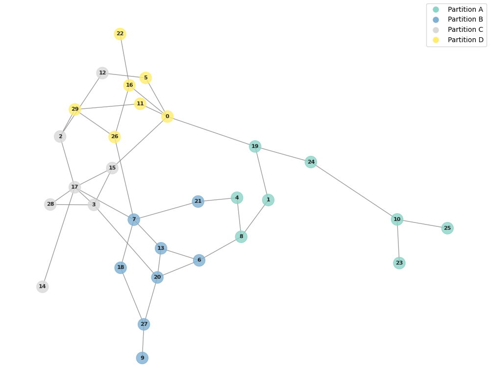
Generated Partitions for a 30-Node Graph with Max Nodes set to 10
QUBO Partitioning Example
For QUBO problems that are too large to solve directly, PartitioningProgramEnsemble can also partition QUBO problems via D-Wave’s hybrid decomposers:
import dimod
import hybrid
from divi.qprog import PartitioningProgramEnsemble
from divi.qprog.problems import BinaryOptimizationProblem
from divi.qprog.optimizers import ScipyOptimizer, ScipyMethod
from divi.backends import MaestroSimulator

bqm = dimod.generators.gnp_random_bqm(25, p=0.5, vartype="BINARY")

problem = BinaryOptimizationProblem(
    bqm,
    decomposer=hybrid.EnergyImpactDecomposer(size=8),
    composer=hybrid.SplatComposer(),
)

ensemble = PartitioningProgramEnsemble(
    problem=problem,
    n_layers=2,
    optimizer=ScipyOptimizer(ScipyMethod.COBYLA),
    max_iterations=10,
    backend=MaestroSimulator(),
)

ensemble.create_programs()
ensemble.run()
solution = ensemble.aggregate_results()
Why Partition?
Quantum hardware is limited in the number of qubits and circuit depth. For large problems:
- Full QAOA is intractable.
- Partitioned QAOA trades global optimality for scalability and parallel execution.
- It enables fast, approximate solutions using many small quantum jobs rather than one large one.
-
Fiedler, M. (1973). Algebraic connectivity of graphs. Czechoslovak Mathematical Journal, 23(2), 298-305. ↩︎
-
Karypis, G., & Kumar, V. (1997). METIS: A software package for partitioning unstructured graphs, partitioning meshes, and computing fill-reducing orderings of sparse matrices. Department of Computer Science and Engineering, University of Minnesota. ↩︎
-
Kernighan, B. W., & Lin, S. (1970). An efficient heuristic procedure for partitioning graphs. The Bell System Technical Journal, 49(2), 291-307. ↩︎